Aggregations

Aggregations build on complex searches, providing faster results and being easier to perform. Several searches are aggregated to be analyzed, computed and displayed as a single request.

Compared to queries, aggregations consume more CPU and memory.

Every aggregation is a combination of one or more buckets and zero or more metrics.

For example, in the query

SELECT COUNT(status_code)
FROM table
GROUP BY status_code

COUNT(status_code) is equivalent to a metric and
GROUP BY status_code is equivalent to a bucket.

Buckets

Buckets create groups of documents based on certain criteria, depending on the aggregation type. The name derives from the concept of gathering documents into containers/buckets. Buckets don’t calculate metrics like metrics do.

For example, the date 2022-12-19 would be in a bucket for December and the city of Campinas, in a bucket for the state of São Paulo.

Buckets can be contained within other buckets. For example, Campinas would be in a bucket for the state of São Paulo and the entire bucket of São Paulo would be in a bucket for Brazil.

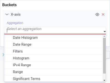
See the table below for a description of the main types of buckets. The image below shows the list from which to choose a bucket type (located in the right side of the Visualize screen). See also how to create a new visualization and learn how to get to this screen to choose the type of buckets.

detail from the Visualize screen showing bucket types

Frequently used bucket types

Type

Definition

Parameters

Histogram

Dynamically groups documents into buckets based on specific intervals (numeric values or numeric range values). It is similar to range aggregation; however, instead of defining each range specifically, you may activate the use auto interval option or enter a number for the minimum range. An example of use for the histogram is to display the number of occurrences of an event (e.g., amount of 400 error responses) for each month.

Minimum interval: Select Use auto interval or specify the minimum interval.

Date histogram

Similar to the regular histogram aggregation, but exclusive for date values or date range values.
The difference to the regular histogram is that date histogram understands the concepts of a calendar (e.g., knows that December has more days than February, differentiates between time zones). Regular Histograms interpret dates as numbers.

Minimum interval: specify the minimum rounding interval. By default, Auto is selected. Other accepted units: millisecond, second, minute, hour, day, week, month and year.

Range

Defines a set of intervals, each representing a bucket. Each document is checked according to the variation range of its interval and grouped according to its relevance or correspondence to this range, which can be numeric, based on date values or on IP address. Usage example: When searching for a certain type of product in an online store, range can display the most popular price range for that type of product.

>=: inform a value for the beginning of the interval
<: inform a value for the end of the interval.

Date range

A range aggregation specific for date values.

Acceptable date formats: inform a start and end for each range.
Example:
from: now-1w/w < now minus 1 week, rounded up to the beginning of the week.
to:now >= now minus 1 week, rounded up to the beginning of the week.

Filters

Aggregation in which each bucket contains documents that match a query. It is possible to define more than one filter.

Filter: provide the search expression. It can be written in DQL or Lucene. Click + Add filter to add another filter.

NOTE: Select Lucene or DQL and use the corresponding syntax. For a query written in Lucene to be interpreted correctly, Lucene must be selected. The same is true for DQL.

Terms

Group by categories and retrieve the total number of documents in each category. That is, terms tells you the number of times a given term appears in your documents.

Order by: defines the ordering type, based on the metric selected, which can be:
Custom metric or
_ Alphabetical_.

Significant terms

Returns occurrences of interesting or unusual terms. The result shown is the difference between the occurrence of a term in every index and the occurrence of the same term in your queries, highlighting the terms that are relevant within each search context. For example, the term "sensedia" would be relevant in the context of "apis".

Size: select how many term buckets should be returned from the total list of terms.

Advanced Parameters

Both metrics and buckets aggregations allow you to add advanced parameters.

To access advanced parameters, click the expand/collapse icon next to Advanced, as shown in the image below.

Depending on the type or field selected for the aggregation, in addition to the JSON input field, different options may be available for entering or selecting data.

animation highlighting the JSON input field

See the table below for definitions and usage examples for the main advanced parameters used with bucket aggregations.

The definitions of each bucket aggregation type and its basic parameters are in the previous table.

Type

Advanced Parameters

Date Histogram

calendar_interval specifies calendar intervals using a name (e.g., month) or unit (e.g., 1M). Amounts like 2M are not supported. 1M and month are equivalent. Accepted units: minute or 1m, hour or 1h, day or 1d, week or 1w, month or 1M, quarter or 1q, year or 1y.
Example: calendar_interval: "1M¨
fixed_interval sets fixed, calendar-independent intervals. Allows multiples of a unit. Months and quarters cannot be defined as fixed intervals because they vary. Supported units: milliseconds ms, seconds s, minutes m, hours h, days d.
Example: "fixed_interval": "30d".
keys Timestamps that represent data are returned in buckets of keys.
key_as_string same timestamp, converted to a string data, whose format is specified in the format parameter.
Example: "key_as_string": "2022-12-19"
time-zone used to indicate a time zone that differs from the default. The default time zone used for storage is UTC.
Example: "time_zone": "-01:00"
offset sets other intervals within the same unit. For example, each bucket with the range day runs from midnight to midnight. Adjusting the offset to +6h, each bucket will go from 6am to 6pm.
Example: "offset": "+6h"
keyed when enabled, associates a single string key with each bucket and returns the intervals as a hash instead of an array.
Example: "keyed": true
order determines how to order the results. Examples: "order": { "key": "asc" }
min_doc_count sets the minimum number of buckets returned. By default, the histogram returns buckets even when the count is zero.
extended_bounds extends the bounds, forcing buckets to be displayed even if they fall before the minimum value or after the maximum value. min_doc_count returns empty buckets, but by default it only returns buckets that are between the minimum and maximum values.

Range and Date range

missing defines how to handle missing values. The default is to ignore such values. In the example below, documents that did not have a value in the date field will be added to the bucket "Older" as they had the value "1976/11/30".
Example:

"missing": "11/30/1976",
"ranges":[
      {
          "key": "Older",
          "to": "2015/01/01"
      },
]

keyed when enabled, associates a single string key with each bucket and returns intervals as a hash instead of an array.
Example: "keyed": true

Filters

other_bucket adds a bucket to the response, gathering all documents that do not match certain filters. Values can be:
false does not add the other bucket,
true returns the bucket with name other (if named filters are being used) or as the last bucket (if anonymous filters are being used).
other_bucket_key used to define another value for the other bucket, different from the default other.
Example: `"other_bucket_key": "other_messages"

Histogram

missing defines how to handle missing values. The default is to ignore such values. In the example below, documents that do not have a value in the quantity field will be added to the same bucket as documents that have the value 0.
Example:

"histogram": {
         "field": "quantity",
         "range": 10,
         "missing": 0
       }

min_doc_count sets the minimum number of buckets for the response. By default, the histogram returns buckets even when the count is zero.
Example: "min_doc_count": 1
extended_bounds extends the limits, forcing buckets to be displayed even if they fall before the minimum value or after the maximum value. min_doc_count returns empty buckets, but by default it only returns buckets that are between the minimum and maximum values.
Example:

"extended_bounds" : {
                 "min" : "2014-01-01",
                 "max" : "2014-12-31"
             }

order establishes the sort order of the results.
Examples: "order": { "_key": "asc" }

Terms and Significant terms

include and exclude filter values for which buckets will be created. include determines which values are "allowed" in the aggregation and exclude determines which values will not be included in the aggregation. include proceeds exclude.
min_doc_count sets the minimum number of results returned with top occurrences. By default it is set to 3. It is recommended not to set it to 1.
Example: "min_doc_count": 10
size sets the quantity returned. By default, the first 10 terms or significant terms are returned, according to the selected order. You can change the size to 0 to get all terms (note, however, that the result can be large and impact CPU and network).
shard_size defines how many documents, at most, should be collected from each shard. By default (-1), this amount is estimated automatically, based on the number of shards and the size parameter. shard_size cannot be smaller than size.
Example: "shard_size": 1000

Metric aggregations

Metrics extract statistics from documents grouped into one or more buckets or from buckets resulting from other aggregations. Generally speaking, metrics generate one or more numbers that describe the grouped documents.

Metrics can be:

Single-value: returns only one metric.
Multi-value: returns more than one metric.

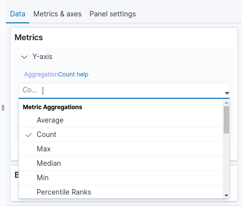
See the table below for a brief description of each metric. The image below shows the part of the Visualize screen where you can select a metric.

"detail from Visualize screen showing metrics selection

Frequently used Metrics aggregation

Metrics

Description

Average

Single-value metrics aggregation that calculates the average of numeric values from documents contained in the buckets. The numeric values can come from histogram fields or other numeric fields.

Count

This metrics aggregation counts the documents present in each of the selected buckets.

Sum

A single-value metrics aggregation that sums the numeric values from documents present in the buckets.

Max

A single-value metrics aggregation that brings the maximum value of numeric values from documents present in the buckets.

Median

A single-value metrics aggregation that calculates the median of numeric values. The median is indicated to be used when there are extremely high or low values (outliers). Median is not affected by an outlier, like the average is.

Min

A single-value metrics aggregation that returns the minimum value of numeric values of documents present in buckets.

Percentiles

A multi-value metrics aggregation that calculates one or more percentiles on numeric values from documents present in the buckets. Percentile is the percentage of data that are equal to or less than a given value within a frequency distribution. The default distribution is [1, 5, 25, 50, 75, 95, 99]. Alternatively, you can choose different values, from 0 to 100. Commonly used to find outliers. This metrics aggregation is an approximation. Usage example: In relation to the number of visits to your web page, display the most common delay and how long the longest response times are.

Percentile ranks

A multi-value metrics aggregation that calculates one or more percentile ranks on numeric values from documents present in the buckets. The percentile rank of a given value is the percentile of values equal to or less than a threshold grouped by a given value. For example, if a value is greater than or equal to 80% of the values, then its percentile rank is 80%. It can be used, for example, in visualizations that monitor the Service Level Agreement (SLA).

Standard deviation

Represents the variation of a group of values around the mean. A low standard deviation indicates that the values tend to be close to the mean or expected value.

Top hits

A multi-value metrics aggregation that ranks the most relevant data. It is recommended to be used as a sub aggregator so that top matching documents can be grouped by buckets. Settings:
- Size: Set the maximum number of top hits per bucket.
- Aggregate with: if the chosen size is greater than 1, define here how the results will be grouped.
- Sort on: specify how the top hits should be sorted.

Unique Count

A single-value metrics aggregation that presents the approximate count of distinct values in a field. It can be used, for example, to view the number of unique IP addresses accessing your service.

Pipeline aggregations

With Pipeline Aggregations you can concatenate aggregations using the results of one aggregation as input to another aggregation.

Pipeline aggregations enable more complex statistical calculations, such as derivatives, cumulative sums, and moving averages.

Parent pipeline: pipeline aggregation in which the results of a parent aggregation are used to calculate new buckets or new aggregations that will be added to existing buckets. The min_doc_count for parent pipeline aggregations must be set to 0, which is the default for histogram aggregations. The metric must be a numeric value.
Sibling pipeline: pipeline aggregation in which the aggregation uses the results of a sibling aggregation to compute a new aggregation that will be at the same level as the sibling aggregation. Necessarily, sibling pipelines must be multi-value and the metric, a numerical value.

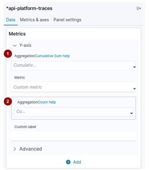
Pipeline aggregations can be found in the same list as the Metrics aggregations, as shown in the image below.

detail of the visualize screen highlighting the list of metrics and pipeline aggregations

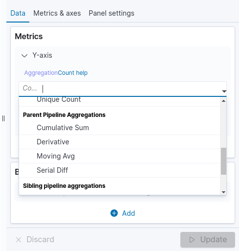
When selecting a pipeline aggregation (identified as 1 in the figure below), whether it is parent or sibling, another box opens so that you can configure the second aggregation (identified as 2 in the figure below).

detail of the visualize screen highlighting the second aggregation configuration area

Parent pipeline aggregations

Aggregation

Description

Cumulative sum

Calculates the cumulative sum of a metric in a parent histogram or parent date histogram aggregation. This aggregation calculates the field value by adding the previous value to the current one. The result will be a single value representing the cumulative sum of the field values. The metric must be numeric and the added histogram must have min_doc_count set to 0 (default value for histogram aggregation).

Derivative

Calculates the derivative of a metric in a parent histogram or date histogram aggregation. The metric must be numeric and the added histogram must have min_doc_count set to 0 (default value for histogram aggregation). Derivatives describe the rate of change in a function. It can be used to identify trends and anomalies in data.

Moving avg

Finds the series of averages of different subgroups (windows) of a dataset. Can be used to smooth out fluctuations or to highlight trends or cycles in time series data.

Serial diff

Serial differencing is a technique that subtracts a value from itself in a time series, at a different interval or period. First, you need to specify a histogram or date histogram for a field. Then you can add a simple metric like sum inside the histogram and add the serial diff to the histogram.

Sibling pipeline aggregations

Aggregation

Description

Average bucket

Calculates the average value of a specified metric in a sibling aggregation. The metric must be numeric and the sibling aggregation must be a multi-bucket aggregation. By default, Auto is selected for the minimum interval. Other supported units: millisecond, second, minute, hour, day, week, month and year.

Max bucket

Identifies the bucket or buckets with the maximum value of a given metric in a sibling aggregation and returns the value and key for that bucket. The metric must be numeric and the sibling aggregation must be a multi-bucket aggregation. Minimum interval:. By default, Auto is selected for the minimum rounding interval. Other supported units: millisecond, second, minute, hour, day, week, month and year.

Min bucket

Identifies the bucket or buckets with the maximum value of a given metric in a sibling aggregation and returns the value and key for that bucket. The metric must be numeric and the sibling aggregation must be a multi-bucket aggregation. Minimum interval: By default, Auto is selected for the minimum rounding interval. Other supported units: millisecond, second, minute, hour, day, week, month and year.

Sum bucket

Calculates the sum across all buckets of a given metric in a sibling aggregation. The metric must be numeric and the sibling aggregation must be a multi-bucket aggregation.

Thanks for your feedback!

EDIT

How useful was this article to you?